Preemptive Precedence CPU Scheduling Algortithm

Prerequisite – https://www.geeksforgeeks.org/cpu-scheduling-in-operating-systems/

Introduction:

It is a pre-emptive methodology of scheduling processes that works based mostly on the precedence of a course of. On this algorithm, the scheduler schedules the duties to work as per the precedence. A better precedence course of ought to be executed first. Once we are having 2 processes with equal priorities then we select to pick the method based mostly on FCFS (First Come First Serve). When it reaches to closing course of then we are going to execute the remaining processes based mostly on precedence.

Notice: Lesser the Quantity, Extra Precedence 

For instance: 1 is excessive precedence, 10 – low precedence

Process:

• Step-1: Choose the primary course of whose arrival time will probably be 0, we have to choose that course of as a result of that course of is just be executing at time t=0.
• Step-2: Verify the precedence of the subsequent accessible course of.

                         Right here we have to test for 3 circumstances.

                         (i) if precedence_{(current_process)} > precedence_{(prior_process)} then execute the present course of.

                         (ii) if precedence_{(current_process)} > precedence_{(prior_process)} then execute the prior course of.

                         (iii) if precedence_{(current_process)} > precedence_{(prior_process)} then execute the method which arrives first i.e., arrival time 

                               ought to be first.

• Step-3: Repeat Step-2 till it reaches the ultimate course of.
• Step-4: When it reaches the ultimate course of, select the method which is having the very best precedence & execute it. Repeat the identical step till all processes completes their execution.

Notice: A Course of is accomplished when its burst time turns into 0.

Instance-1: Contemplate the next desk of arrival time, Precedence and burst time for 5 processes P1, P2, P3, P4 and P5. 

Course of	Arrival Time	Precedence	Burst Time
P1	0 ms	3	3 ms
P2	1 ms	2	4 ms
P3	2 ms	4	6 ms
P4	3 ms	6	4 ms
P5	5 ms	10	2 ms

Working: (for input-1):

Step-1:  At Arrival time t = 0, course of P1 is executed for 1ms as its arrival time is from 0ms to 1ms, as it’s the first course of within the prepared queue. Remaining Burst time (B.T) for P1 = 3-1 = 2 ms.

Step-2: At time t = 1, course of P2 is having larger precedence than P1, so we have to execute Course of P2, for 1ms.
             Remaining B.T for P2 = 4-1 = 3 ms.

Step-3: At time t = 2, Course of P2 is having larger precedence than P3, So once more P2 will probably be executed for 1 ms.
             Remaining B.T for P2 = 3-1 = 2 ms.

Step-4: At time t = 3, Course of P2 is having larger precedence than P4, So P2 now will execute for two ms because the arrival time of P4 is from 3 ms to five ms. Remaining B.T for P2 = 2-2 = 0 ms.

             -> Right here Course of P2 is accomplished with its execution because the burst time for P2 is 0.
             -> Right here the Arrival time for Processes is now 5 so it has reached to all of the Processes.

Step-5: Now we have to schedule the method with the very best precedence, Right here we’re having P1 as the very best precedence, So P1 is executed utterly and the remaining B.T of P1 = 2-2 = 0 ms.

Step-6: Equally repeat Step-5 for all of the remaining processes based mostly on precedence till all processes full their execution.

Gantt chart:

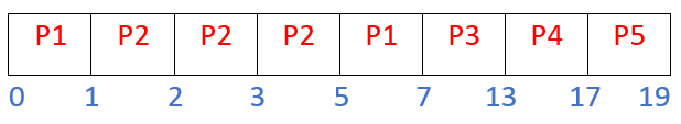
Now we have to calculate the completion time (C.T) & First Arrival Time (F.A.T) of every course of by way of Gantt chart.

C.T -> P1-7 ms, P2-5 ms, P3-13 ms, P4-17 ms, P5-19 ms.
F.A.T -> P1-0 ms, P2-1 ms, P3-7 ms, P4-13 ms, P5-17 ms.

Flip Round Time (T.A.T) = (Completion Time) – (Arrival Time)

Ready Time (W.T) = (Flip Round Time) – (Burst Time)

Response Time (R.T) = (First Arrival Time) – (Arrival Time)

After calculating the above fields, the ultimate desk appears like

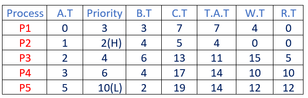
Right here, H – Increased Precedence L – Least Precedence

Output :

Whole Flip Round Time = 7 + 4 + 11 + 14 + 14 = 50 ms
Common Flip Round Time = (Whole Flip Round Time)/(no. of processes) = 50/5 = 10.00 ms

Whole Ready Time = 4 + 0 + 15 + 10 + 12 = 41 ms
Common Ready Time = (Whole Ready Time)/(no. of processes) = 41/5 = 8.20 ms

Whole Response Time = 0 + 0 + 5 + 10 + 12 = 27 ms
Common Ready Time = (Whole Ready Time)/(no. of processes) = 27/5 = 5.40 ms

Instance 2: 

Contemplate the next desk of arrival time, Precedence and burst time for seven processes P1, P2, P3, P4, P5, P6 and P7

Course of	Arrival Time	Precedence	Burst Time
P1	0 ms	3	8 ms
P2	1 ms	4	2 ms
P3	3 ms	4	4 ms
P4	4 ms	5	1 ms
P5	5 ms	2	6 ms
P6	6 ms	6	5 ms
P7	10 ms	1	1 ms

Working: (for input-2)

Step-1: At time t = 0, Course of P1 is offered within the prepared queue, executing P1 for 1 ms. 
             Remaining B.T for P1 = 8-1 = 7 ms.

Step-2: At time t = 1, the precedence of P1 is larger than P2, so we execute P1 for two ms, because the arrival time of P2 is from 1 ms to three ms.                  Remaining B.T for P1 = 7-2 = 5 ms.

Step-3: At time t = 3, the precedence of P1 is larger than P3, so we execute P1 for 1 ms.
             Remaining B.T for P1 = 5-1 = 4 ms.

Step-4: At time t = 4, the precedence of P1 is larger than P4, so we execute P1 for 1 ms.
             Remaining B.T for P1 = 4-1 = 3 ms.

Step-5: At time t = 5, the precedence of P5 is larger than P1, so we execute P5 for 1 ms.
             Remaining B.T for P5 = 6-1 = 5 ms.

Step-6: At time t = 6, the precedence of P5 is larger than P6, so we execute P5 for 4 ms.
             Remaining B.T for P5 = 5-4 = 1 ms.

Step-7: At time t = 7, the precedence of P7 is larger than P5, so we execute P7 for 1 ms.
             Remaining B.T for P7 = 1-1 = 0 ms.
             -> Right here Course of P7 completes its execution.

Step-8: Now we take the method which is having the very best precedence. Right here we discover P5 is having the very best precedence & execute P5 utterly and the remaining B.T of P5 = 1-1 = 0 ms.

Step-9: Equally repeat Step-8 for all of the remaining processes based mostly on precedence till all processes completes their execution.

Gantt chart:

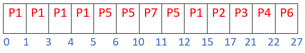
Now we have to calculate the completion time (C.T) & First Arrival Time (F.A.T) of every course of by way of Gantt chart.

C.T -> P1-15 ms, P2-17 ms, P3-21 ms, P4-22 ms, P5-12 ms, P6-27 ms, P7- 11 ms.

F.A.T -> P1-0 ms, P2-15 ms, P3-17 ms, P4-21 ms, P5-5 ms, P6-22 ms, P7-10 ms.

Flip Round Time (T.A.T) = (Completion Time) – (Arrival Time)

Ready Time (W.T) = (Flip Round Time) – (Burst Time)

Response Time (R.T) = (First Arrival Time) – (Arrival Time)

After calculating the above fields, the ultimate desk appears like

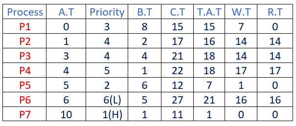
Right here, H – Increased Precedence, L – Least Precedence

Output:

Whole Flip Round Time = 15 + 16 + 18 + 18 + 7 + 21 + 1 = 96 ms
Common Flip Round Time = (Whole Flip Round Time)/(no. of processes) = 96/7 = 13.71 ms

Whole Ready Time = 7 + 14 + 14 + 17 + 1 + 16 + 0 = 69 ms
Common Ready Time = (Whole Ready Time)/(no. of processes) = 69/7 = 9.85 ms

Whole Response Time = 0 + 14 + 14 + 17 + 0 + 16 + 0 = 61 ms
Common Ready Time = (Whole Ready Time)/(no. of processes) = 61/7 = 8.71 ms

Drawbacks of Pre-emptive Precedence Scheduling Algorithm:

Hunger Drawback: That is the issue through which a course of has to attend for an extended period of time to get scheduled into the     CPU. This situation known as the hunger downside.

Instance: In Instance 2, we are able to see that course of P1 is having Precedence 3 and we’ve pre-empted the method P1 and allotted the CPU to P5. Right here we’re solely having 7 processes.

Now, if suppose we’ve many processes whose precedence is larger than P1, then P1 wants to attend for an extended time for the opposite course of to be pre-empted and scheduled by the CPU. This situation known as as hunger downside.

Answer: The answer for this Hunger downside is Ageing.

Growing old: This may be executed by decrementing the precedence quantity by a sure variety of a specific course of which is ready for an extended time frame after a sure interval.

Instance: After each 3 items of time, all of the processes that are in ready state, the precedence of these processes will probably be decreased by 2, So, if there’s a course of P1 which is having precedence 5, after ready for 3 items of time its precedence will probably be decreased from 5 to three in order that if there’s any course of P2 which is having precedence as 4 then that course of P2 will wait and P1 will probably be scheduled and executed.

The implementation of this scheduling course of is supplied on this article.